There is a class of systems in nature for which the spatiotemporal evolution can be described using a master type of equation. While chemical reactions at surfaces is one of them, it is not limited to those.
The master equation imposes that
given a probability distribution  over states, the probability distribution at one
infinitesimal time
over states, the probability distribution at one
infinitesimal time  later can be
obtained from
later can be
obtained from
where the important bit is that each  only depends on the state just before the current state.
The matrix
only depends on the state just before the current state.
The matrix  consists of constant real entries,
which describe the rate at which the system can propagate
from state
consists of constant real entries,
which describe the rate at which the system can propagate
from state  to state
  .
In other words the system is without memory which is
usually known as the Markov approximation.
.
In other words the system is without memory which is
usually known as the Markov approximation.
Kinetic Monte Carlo (kMC) integrates this equation
by generating a state-to-state trajectory using a
preset catalog of transitions or elementary steps
and a rate constant for each elementary step. The reason
to generate state-to-state trajectories rather than just
propagating the entire probability distribution at once
is that the transition matrix easily becomes
too large for many systems at hand that even storing it
would be too large for any storage device in foreseeable
future.
As a quick estimate consider a system with 100
sites and 3 possible states for each site, thus having
 different configurations. The matrix
to store all transition elements would have
different configurations. The matrix
to store all transition elements would have
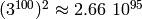 entries, which
exceeds the number of atoms on our planet by roughly 45 orders of
magnitude. [1] And even though most of these elements
would be zero since the number of accessible states is
usually a lot smaller, there seems to be no simple
way to transform to and solve this irreducible matrix
in the general case.
entries, which
exceeds the number of atoms on our planet by roughly 45 orders of
magnitude. [1] And even though most of these elements
would be zero since the number of accessible states is
usually a lot smaller, there seems to be no simple
way to transform to and solve this irreducible matrix
in the general case.
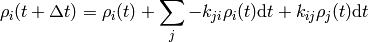
Thus it is a lot more feasible to take one particular configuration and figure out the next process as well as the time it takes to get there and obtain ensemble averages from time averages taken over a sufficiently long trajectory. The basic steps can be described as follows
- Fix rate constants
initial state
, and initial time
while
do
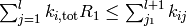
- draw random numbers
- find
such that
- increment time
end
Let’s understand why this simulates a physical process.
The Markov approximation mentioned above implies several things:
not only does it mean one can determine the next process from
the current state. It also implies that all processes happen
independently of one another because any memory of the system
is erased after each step. Another great simplification is
that rate constants simply add to a total rate, which is
sometimes referred to as
Matthiessen’s rule,
viz the rate with which any process occurs is simply
 .
.
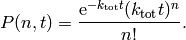
First, one can show that the probability that  such processes
occur in a time interval
such processes
occur in a time interval  is given by a Poisson distribution [2]
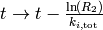
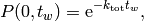
The waiting time or escape time  between two such processes
is characterized by the probability that zero such processes have occured
between two such processes
is characterized by the probability that zero such processes have occured
(1)
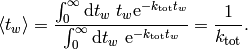
which, as expected, leads to an average waiting time of
Therefore at every step, we need to advance the time by a random number that
is distributed according to (1). One can obtain such a random
number from a uniformly distributed random number ![R_2\in ]0,1]](../_images/math/2b61dc75797e588cb22ee51d57a7cfbedbe325ca.png) via
via  . [3]
. [3]
Second, we need to select the next process. The next process occurs randomly but if we did this a very large number of times for the same initial state the number of times each process is chosen should be proportional to its rate constant. Experimentally one could achieve this by randomly sprinkling sand over an arrangement of buckets, where the size of the bucket is proportional to the rate constant and count each hit by a grain of sand in a bucket as one executed process. Computationally the same is achieved by steps 2 and 3.
For a very practical introduction I recommend Arthur Voter’s tutorial [4]
and Fichthorn [5] for a derivation, why is chosen they
way it is. The example given there is also an excellent exercise for
any beginning kMC modeler. For recent review on implementation techniques
I recommend the review by Reese et al. [6] and for a review over status
and outlook I recommend the one by Reuter [7] .
| [1] | Wolfram Alpha’s estimate for number of atoms on earth. |
| [2] | C. Gardiner, 2004. Handbook of Stochastic Methods: for Physics, Chemistry, and the Natural Sciences. Springer, 3rd edition, ISBN:3540208828. |
| [3] | P. W. H, T. S. A, V. W. T, and F. B. P, 2007 Numerical Recipes 3rd Edition: The Art of Scientific Computing. Cambridge University Pres, 3rd edition, ISBN:0521768589, p. 287. link |
| [4] | Voter, Arthur F. “Introduction to the Kinetic Monte Carlo Method.” In Radiation Effects in Solids, 1–23, 2007. http://dx.doi.org/10.1007/978-1-4020-5295-8_1. link |
| [5] | Fichthorn, Kristen A., and W. H. Weinberg. “Theoretical Foundations of Dynamical Monte Carlo Simulations.” The Journal of Chemical Physics 95, no. 2 (July 15, 1991): 1090–1096. link |
| [6] | Reese, J. S., S. Raimondeau, and D. G. Vlachos. “Monte Carlo Algorithms for Complex Surface Reaction Mechanisms: Efficiency and Accuracy.” Journal of Computational Physics 173, no. 1 (October 10, 2001): 302–321. link |
| [7] | Reuter, Karsten. “First-principles Kinetic Monte Carlo Simulations for Heterogeneous Catalysis: Concepts, Status and Frontiers”. Wiley-VCH, 2009. link |
![R_{1}, R_{2} \in ]0,1]](../_images/math/e09ea7a6eb86738fa7845008092520f8346eaa83.png)